Overview
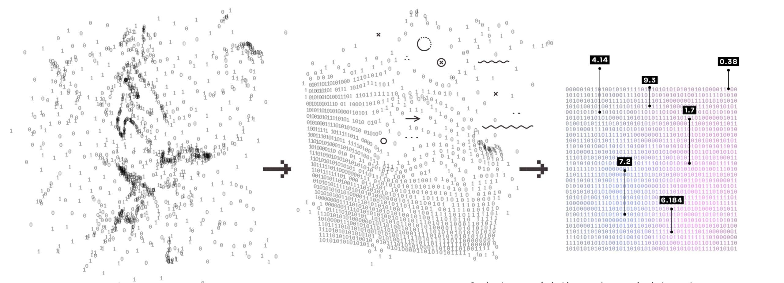
One of the things you realize quickly going from guides, classes, and tutorials into hands-on machine learning projects is that real data is messy. There’s a lot of work to do befor e you even start considering models, performance, or output. Machine learning programs follow the “garbage in, garbage out” principle; if your data isn’t any good, your models won’t be either. This doesn’t mean that you’re looking to make your data pristine, however. The goal of pre-processing isn’t to support your hypothesis, but instead to support your experimentation. In this post, we’ll examine the steps that are most commonly needed to clean up your data, and how to perform them to make genuine improvements in your model’s learning potential.
Handling Missing Values
The most obvious form of pre-processing is the replacement of missing values. Frequently in your data, you’ll find that there are missing numbers, usually in the form of a NaN flag or a null. This could have been because the question was left blank on your survey, or there was a data entry issue, or any number of different reasons. The why isn’t important; what is important is what you’re going to do about it now.
I’m sure you’ll get tired of hearing me say this, but there’s no one right answer to this problem. One approach is to take the mean value of that row. This has the benefit of creating a relatively low impact on the distinctiveness of that feature. But what if the values of that feature are significant? Or have a wide enough range, and polarized enough values, that the average is a poor substitute for what would have been the actual data? Well, another approach might be to use the mode of the row. There’s an argument for the most common value being the most likely for that record. And yet, you’re now diminishing the distinctiveness of that answer for the rest of the dataset.
What about replacing the missing values with 0? This is also a reasonable approach. You aren’t introducing any ‘’new” data to the data set, and you’re making an implicit argument within the data that a missing value should be given some specific weighting. But that weighting could be too strong with respect to the other features, and could cause those rows to be ignored by the classifier. Perhaps the most ‘pure’ approach would be to remove any rows that have any missing values at all. This too is an acceptable answer to the missing values problem, and is also one that maintains the integrity of the data set, but it is frequently not an option depending on how much data you have to give up with this removal.
As you can see, each approach has its own argument for and against, and will impact the data in its own specific way. Take your time to consider what you know about your data before choosing a NaN replacement, and don’t be afraid to experiment with multiple approaches.
Normalization and Scaling
As we discussed in the above section with the 0 case, not all numbers were created equal. When discussing numerical values within machine learning, people often refer to numerical values instead as “continuous values”. This is because numerical values can be treated as having a magnitude and distance from each other (ie, 5 is 3 away from 2, is more than double the magnitude of 2, etc). The importance of this lies in the math of any sort of linearly based or vector based algorithm. When there’s a significant difference between two values mathematically, it creates more distance between the two records in the calculations of the models.
As a result, it is vitally important to perform some kind of scaling when using these algorithms, or else you can end up with poorly “thought out” results. For example: one feature of a data set might be number of cars a household owns (reasonable values: 0-3), while another feature in the data set might be the yearly income of that household (reasonable values: in the thousands). It would be a mistake to think that the pure magnitude of the second feature makes it thousands of times more important than the former, and yet, that is exactly what your algorithm will do without scaling.
There are a number of different approaches you can take to scaling your numerical (from here on out, continuous) values. One of the most intuitive is that of min-max scaling. Min-max scaling allows you to set a minimum and maximum value that you would like all of your continuous values to be between (commonly 0 and 1) and to scale them within that range. There’s more than one formula for achieving this, but one example is:
X’ = ( ( (X – old_min) / (old_max – old _min) ) * (new_max – new_min) ) + new_min
Where X’ is your result, X is the value in that row, and the old_max/min are the minimum and maximum of the existing data.
But what if you don’t know what minimum and maximum values you want to set on your data? In that case, it can be beneficial to use z-score scaling. Z-score scaling is a scaling formula that gives your data a mean of 0 and a standard deviation of 1. This is the most common form of scaling for machine learning applications, and unless you have a specific reason to use something else, it’s highly recommended that you start with z-score.
The formula for z-score scaling is as follows:
X’ = (X – mean) / standard_deviation
Once your data has been z-score scaled, it can even be useful to ‘normalize’ it by applying min-max scaling on the range 0-1, if your application is particularly interested in or sensitive to decimal values.
Categorical Encoding
We’ve focused entirely on continuous values up until now, but what about non-continuous values? Well, for most machine learning libraries, you’ll need to convert your string based or “categorical” data into some kind of numerical representation. How you create that representation is the process of categorical encoding, and there are – again – several different options for how to perform it.
The most intuitive is a one-to-one encoding, where each categorical value is assigned with and replaced by an integer value. This has the benefit of being easy to understand by a human, but runs into issues when being understood by a computer. For example: Let’s say we’re encoding labels for car companies. We assign 1 to Ford, 2 to Chrysler, 3 to Toyota, and so on. For some algorithms, this approach would be fine, but for any that involve distance computations, Toyota now has three times the magnitude that Ford does. This is not ideal, and will likely lead to issues with your models.
Instead, it could be useful to try to come up with a binary encoding, where certain values can be assigned to 0 and certain values can be assigned to 1. An example might be engine types, where you only care if the engine is gas powered or electric. This grouping allows for a simple binary encoding. If you can’t group your categorical values however, it might be useful to use what’s called ‘one-hot encoding’. This type of encoding converts every possible value for a feature into its own new feature. For example: the feature “fav_color” with answers “blue”, “red”, and “green”, would become three features, “fav_color_blue”, “fav_color_green”, and “fav_color_red”. For each of those new features, a record is given a 0 or a 1, depending on what their original response was.
One-hot encoding has the benefits of maintaining the most possible information about your dataset, while not introducing any continuous value confusion. However, it also drastically increases the number of features your dataset contains, often with a high cost to density. You might go from 120 categorical features with on average 4-5 answers each, to now 480-600 features, each containing a significant number of 0s. This should not dissuade you from using one-hot encoding, but it is a meaningful consideration, particularly as we go into our next section.
Feature Selection
Another way in which your data can be messy is noise. Noise, in a very general sense, is any extraneous data that is either meaningless or confuses your model. As the number of features in your model increases, it can actually become harder to distinguish between classes. For this reason, it’s sometimes important to apply feature selection algorithms to your dataset to find the features that will provide you with the best models.
Feature selection is a particularly tricky problem. At its most simple, one can just remove any features that contain a single value for all records, as they will add no new information to the model. After that, it becomes a question of calculating the level of mutual information and/or independence between the features of your data. There are many different ways to do this, and the statistical underpinnings are too dense to get into in the context of this blog post, but several machine learning libraries will implement these functions for you, making the process a little easier.
Outlier Removal
The other main form of noise in your data comes from outliers. Rather than a feature causing noise across multiple rows, an outlier occurs when a particular row has values that are far outside the “expected” values of the model. Your model, of course, tries to include these records, and by doing so pulls itself further away from a good generalization. Outlier detection is its own entire area of machine learning, but for our purposes, we’re just going to discuss trying to remove outliers as part of pre-processing for classification.
The simplest way to remove outliers is to just look at your data. If you’re able to, you certainly can by hand select values for each feature that are beyond the scope of the rest of the values. If there are too many records, too many features, or you want to remain blind and unbiased to your dataset, you can also use clustering algorithms to determine outliers in your data set and remove them. This is arguably the most effective form of outlier removal, but can be time consuming as you now have to build models in order to clean your data, in order to build your models.
Conclusion
Pre-processing may sound like a straightforward process, but once you get into the details it’s easy to see its importance in the machine learning process. Whether its preparing your data to go into the models, or trying to help the models along by cleaning up the noise, pre-processing requires your attention, and should always be the first step you take towards unlocking the information in your data.


