
In our introductory blog piece, we discussed some high level statistical concepts which you can read HERE if you haven’t already or need a quick refresher. Now, we can finally start to dive more into the data and start running some tests.
Correlation: A First Clue for a Relationship
 A good place to start data analysis is by looking at correlation. Correlation, typically denoted as r in statistics language, is the relationship between the independent variable, x, and the dependent variable, y, and lies in between -1 and 1. Put even more simply, correlation tells us if there is a relationship occurring between two variables.
This is an important statistical concept, because it sets the stage for further investigation with our data. Finding the correlation between two values is our first clue that a relationship either exists, or does not exist, between the two variables. Using our knowledge about the strength of the relationship, we can then proceed to find out how good one is at predicting the other using linear regression methods. Essentially, correlation is the groundwork that allows us to determine which relationships are worth further investigation. Our correlation value can provide valuable insight on the strength and the direction of the relationship.
Below is a comprehensive table that you can use to decode your correlation value:
| CHARACTERISTIC | INTERPRETATION |
| Positive correlation value | Positive direction / association; as one variable increases, so does the other |
| Negative correlation value | Negative direction / association; as one variable increases, the other decreases |
| |r| is closer to 1 | The closer |r| is to one, the stronger the association |
| |r| closer to 0 | The closer |r| is to zero, the weaker the association |
Finding our correlation value, and many other statistical tools, is made easy in Excel. The function you will use to find r is: =CORREL(array1, array2). Array 1 will simply be all of the data for your first variable, and array 2 is all of the data for our second variable; the order is negligible. For example, if I was finding the correlation between GPA and SAT scores, I would first select all of my GPA data points, and then I would separate it from the second array with a comma, and then select all of my SAT data points. Then you press enter and voila! You have your correlation value.
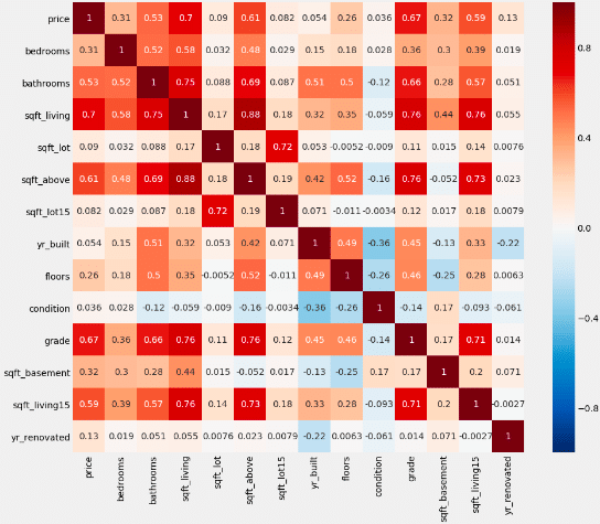
Going back to our example data set, we have created a correlation table that shows the correlation between all of our different variables. A heat map has been included on top to help visually show which have strong or weak associations and which have positive or negative associations. The more saturated the coloring of the box, the stronger the association. If the box is more red, the association is positive, and if the box is more blue, the association is negative. For example, a dark red box would indicate a strong, positive correlation, or a lighter blue would indicate a weak, negative correlation.
Perhaps the most important thing to take away from this section is that correlation does NOT imply causation. Two variables may be correlated, but that does not mean that one causes the other; we cannot emphasize this enough. There may be other confounding variables, which are variables that are not accounted for, that may be the cause of the phenomena that we see. For example, let’s say you find there is a correlation between water consumption and the frequency of illness. It would absolutely ludicrous to draw the conclusion that drinking water causes you to be ill! Instead, we would use this finding of correlation to indicate that there is likely something else going on, such as the presence of cholera. While there is a correlation between the water consumption and illness, we know that the consumption of water isn’t truly what is causing the illnesses; it is the infectious bacteria that is contaminating the water that is causing people to become ill. This is why it is important to discern the difference between correlation and causation so you do not inaccurately report findings. Statistics lays down the ground works for your analysis, but proper research is necessary to really come to the true root of the phenomena.
AB Hypothesis Testing: A Statistical Experiment
Think of the science experiments that you used to do back in school. You pose a question that you are trying to answer; for example, how does sunlight affect plant growth? Then, you make an educated guess, or a hypothesis, as to what you think the results would be, and test whether or not your guess is correct. Statistical hypothesis testing is exactly the same; essentially, you think that there is some kind of relationship occurring between two variables, so you run a statistical experiment to see if your guess, or hypothesis, is correct.
This process begins by looking at the correlation value, which will indicate whether or not there are variables worth investigating. For example, there was a high correlation between the grade, the size of the living room, and the square footage of the house above ground. Since the square footage of the house above ground and the size of the living room can take on an infinite number of values, that makes them continuous variables; this means that it would be advantageous to use linear regression to look deeper into their relationship with price, and even investigate if they can be used to predict it. However, the housing grade is a discrete variable, since there are a finite number of values that this variable can take. You cannot receive a housing grade of 2.5, only 2 or 3. Since grade is a discrete variable, it cannot be used in a linear regression model and would be tested best with the AB hypothesis testing method.
From here, we are going to make a claim that we are trying to prove with the data; this is going to be the alternative hypothesis. However, a null hypothesis also needs to be set, which is a statement that essentially says that our inquiry was wrong, and the data does not support the claim made by the alternative hypothesis. However, the claim cannot be verified by just looking at the raw data; we will need a metric. The metric that is used to numerically show statistical significance is p-value. If you are statistics junkie, read our “For Statistics Junkies” section to learn more about the concepts behind p-value and how it shows us significance; if not, you can go ahead and skip it.
For Statistics Junkies : The “p” in p-value stands for probability, which is what we are actually trying to find during a hypothesis test. What is that probability exactly? It is the probability that we see the value we observe in our data, given that the null hypothesis is true. Put more simply, we have found some observed value in our data set, so what is the probability that we see that observation if the null hypothesis were true. If the p-value is small, that means that the probability of seeing that observation is low if the null hypothesis were actually true. If the p-value is large, that means that the probability of seeing that observation is high if the null hypothesis were actually true. When we say we are doing a test under the assumptions of the null hypothesis, all we are saying is that the test is conducted under the assumption that the null hypothesis is true, which really only affects how we interpret our p-value.
If it is unlikely that we see an observation assuming the null hypothesis to be true, we can conclude that the null hypothesis is false, and there is sufficient evidence in the data to reject it. However, if it is likely that we do see an observation assuming the null is true, we would fail to reject the null hypothesis. Notice how we said fail to reject and not simply accept it. When we fail to reject the null hypothesis, we aren’t saying the null hypothesis is true; we are only saying that there isn’t enough evidence in the data to support the alternative hypothesis claim.
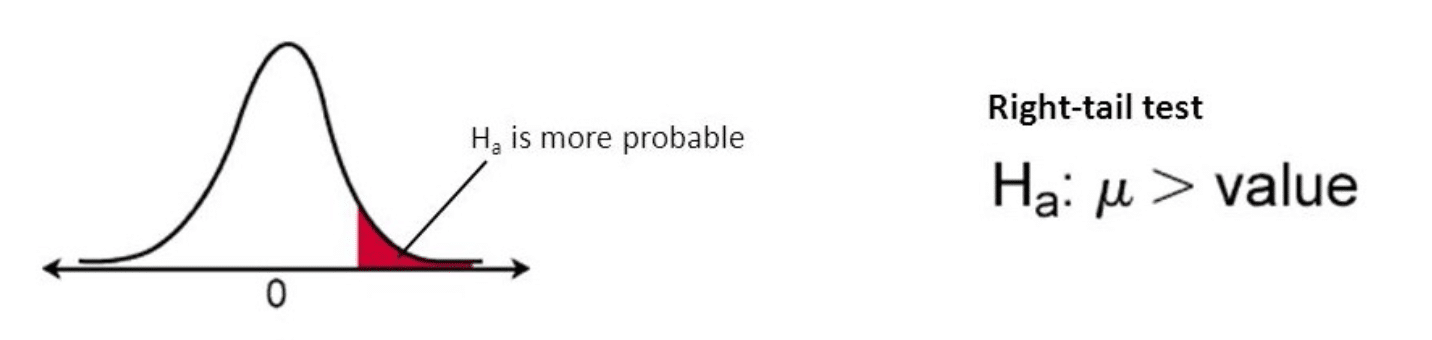
Since we know that when we are finding probability, we also know we are finding an area under the curve. The figure below provides a visual of the area we are trying to find for our example hypothesis test with housing price.
To conduct the hypothesis testing on housing grade, the data was first sectioned off so that group one contained houses grades 7 through 13, and then group two contained houses grades 1 through 6. Note that on the grading scale, a grade of 1 is the lowest and a grade of 13 is the highest. Before conducting any portion of the hypothesis test, it is important to first establish a null and alternative hypothesis:
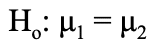
- Null Hypothesis: There is no statistically significant difference between the price of homes with a grade between 7 and 13 and the price of homes with a grade between 1 and 6.
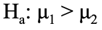
- Alternative Hypothesis: The price of homes with a grade between 7 and 13 is statistically significantly greater than the price of homes with a grade between 1 and 6.
Statistically, this is how to express the null and alternative hypothesis:
- Null Hypothesis:
- Alternative Hypothesis:
When translating statistic language, the actual letters being used to represent variables actually reveal a lot of information. When a Greek letter is used, that means it represents a population parameter. When a Latin letter is used, which is just the alphabet used for modern English, that means it represents a statistic from the sample. For example, “σ” represents the population standard deviation whereas “s” represents the standard deviation of the sample.
Here is a brief overview of the process of hypothesis testing. Following this portion, this process is applied to the housing data to investigate if houses graded 7 through 13 are priced higher than houses graded 1 through 6.
-
Find the test statistic with the following formula:
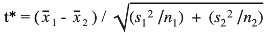
 = the mean price of houses with grades 7-13
 = the mean price of houses with grades 1-6
 = the standard deviation of the price of houses with grades 7-13
 = the standard deviation of the price of the houses with grades 1-6
- n = sample size for each group respectively
- NOTE: In Excel, =STDEV.S must be used when finding s1 and s2 since the standard deviation is being calculated from a sample, not a population
- Calculate p-value with the following formula
- p-value = 1- T.DIST(t*, df, 1)
- This T.DIST function will take a test statistic and find the corresponding area under the curve, or in other words the p-value
- df = degrees of freedom = n-2 where n is the sample size for the entire data set
- NOTE: You must do 1-T.DIST(t*,1) because Excel functions take the area to the LEFT. Since the hypothesis test is one sided in the right direction, you need to take the area to the left and subtract it from 1 to leave us with the remaining area to the right. Note that if the hypothesis test was two sided, then you would multiply T.DIST(t*,1) by 2 since you need to find two areas under the curve.
- p-value = 1- T.DIST(t*, df, 1)
Here is the process applied to the example data set:
- Test Statistic
- t* = (541096.73 – 531672.72) /
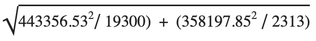
- t* = 1.1631
- t* = (541096.73 – 531672.72) /
- P-Value
- df = 21613 – 2 = 21611
- p-value = 1-T.DIST(1.1631, 21611, 1)
- p-value = 0.12
When following this procedure, the p-value works out to be 0.12. Since this is greater than the standard cut off of 0.05, we would fail to reject the null hypothesis. This does not mean that the alternative hypothesis is to be rejected; it means that there is simply not enough evidence to support the claim that houses with grades 7-13 are priced higher than houses with grades 1-6.
However, it should be noted that this does not express the magnitude of the difference, or lack of difference, in the prices. This is where practical significance comes in. In order to see the actual magnitude of the difference in prices, a confidence interval will be calculated. Essentially, this shows us how different these prices actually are, and if they are subjectively different enough to be noteworthy.
Explanation of Confidence Intervals
Confidence intervals are ranges in which the true population parameter lies. These compliment hypothesis tests perfectly; the hypothesis test will indicate whether or not there is statistical significance, and then the confidence interval will give the magnitude of this significance. For example, if there is a statistical significance between the price of pencils sold at Walmart versus Target, calculating a confidence interval gives a range between which the true difference in prices lies. If it is found that the difference in prices is somewhere between $0.10 and $0.25, it can be said that the findings are not practically significant. However, if it is found that the difference in prices is somewhere between $2.00 and $3.00, it can be argued that that demonstrates practical significance and thus relevance for intended audiences such as consumers.
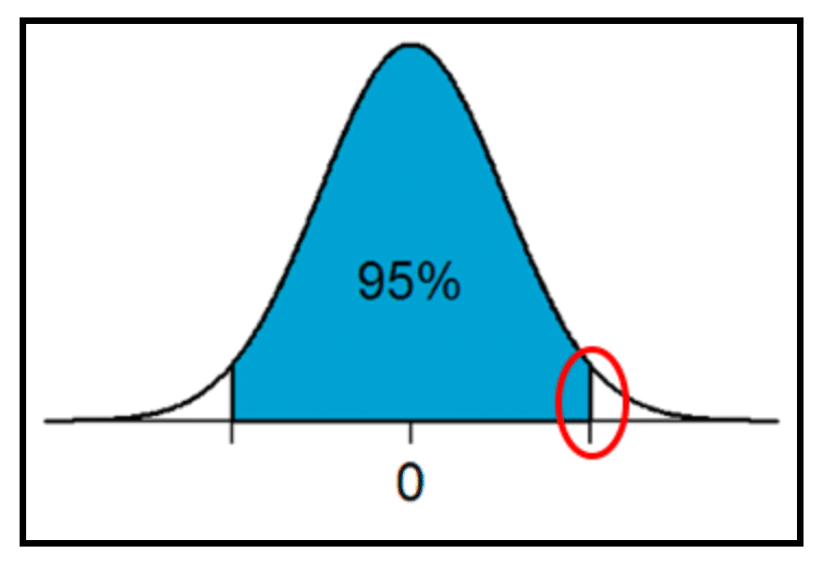
Confidence intervals are conducted at various levels of confidence, indicating the probability that the true population parameter lies within the range. To be more technical, the confidence level says that we have x% confidence that the true population parameter lies within this range. The standard confidence level is 95%, which will be used for this example. When the confidence level is increased, the confidence interval will become wider. When the confidence level is decreased, the confidence interval will become narrower. This will be demonstrated later with the example data with reasoning as to why this logically makes sense.
Here is a visual representation of the task at hand where the red circle represents the multiplier value to first be found:
Here is a brief outline of how to find the confidence interval:
- Find the multiplier, t*
- This is NOT the same t* that used during hypothesis testing; it is a different multiplier that is found separately
- The opposite of the T.DIST function is used, which is T.INV(t*, df). This takes a probability / an area and degrees of freedom, and calculates the corresponding t* value. Referring back up to the figure above, since the t* value to be found includes ALL of the area to the left, the remaining area under the curve needed to be calculated and then added to 0.95. The area under the curve must add up to 1, so therefore the remaining two sections must equal 0.5; due to the symmetrical nature of the bell curve, the two areas on either tail are equal, meaning they are each 0.025. The 0.025 is added to 0.95 to get a total area of 0.975; this will be the area used in the function to find t*.
- Find the margin of error
- Margin of error = (t*) * standard error
- Where standard error =
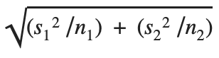
- Where standard error =
- Margin of error = (t*) * standard error
- Add and subtract the margin of error to the difference in sample means
Here the process worked out with the example housing data:
- T-Multiplier
- t* = T.INV(0.975, 21611)
- t* = 1.960074
- Margin of Error
- Standard error =
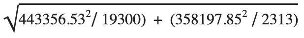 = 8102.85
 - Margin of error = 1.960074 * 8102.85= 15882.17
- Lower Bound = (541096.73 – 531672.31) – 15882.17 = -$6,457.75
- Upper Bound =(541096.73 – 531672.31) + 15882.17 = $25,306.59
- Confidence Interval = (-$6,457.75, $25,306.59)
- Standard error =
When going through this process with the data set, it indicates that the difference between the two groups of homes is somewhere between -$6,457.75 and $25,306.59, where a negative number indicates that group two is actually priced higher than group one. Practical significance is much more subjective than statistical significance, so this price difference may not matter to some people, but it may to others. It should also be noted that the results of the confidence interval actually bolster the results found in the hypothesis test. In the hypothesis test, it was concluded that there is not enough evidence to support the claim that houses with grades 7-13 are priced higher than houses with grades 1-6. Looking at the CI, notice that the interval contains zero, meaning that there is a chance that the two groups of homes are in fact priced the same. It also includes negative numbers, indicating that it is possible that the houses with grades 1-6 are even priced higher than houses with grades 7-13. This bolsters the findings from the hypothesis testing, indicating once again that the null hypothesis should fail to be rejected. However, if the CI did not contain zero within the interval, that means that there it not a chance the prices are the same, and therefore the null hypothesis could be rejected. This is another way that confidence intervals are used to compliment and bolster the findings in hypothesis testing.
Following the same procedures outlined above, the CI was recalculated by decreasing the confidence level to 90% and then increased to 99%:
| CONFIDENCE LEVEL | LOWER BOUND | UPPER BOUND |
| 90% | -$3,904.14 | $22,752.99 |
| 95% | -$6,457.75 | $25,306.59 |
| 99% | -$11,448.97 | $30,297.81 |
When the confidence level was increased, the CI widened. Intuitively, this makes sense since we can be more confident that the population parameter lies somewhere within this range since it contains so many possible values. The root of this is because more possible error is being accounted for as a result of a larger margin of error.
To conclude, it has been identified that there is not a statistically significant difference between the price of homes with grades 7-13 and the price of homes with grades 1-6. Therefore, the null hypothesis fails to reject, as there is insufficient evidence from the data to support the claim that higher graded houses are priced higher. We have 95% confidence that the difference in price between the two housing groups is between -$6,457.75 and $25,306.59.
This process is easily repeatable, especially with tools like Excel, and therefore can be used to investigate numerous variables and characteristics in the data. Here is a comprehensive table of the results from the hypothesis testing with the housing data set:
| VARIABLE | SIGNIFICANCE | CONFIDENCE INTERVAL |
| Waterfront | Statistically significant | (958246.81, 1302378.04) |
| Renovation* | Statistically significant | (190329.86, 269706.56) |
| Renovation Year** | Statistically significant | (35718.74, 192890.85) |
| Condition*** | Not statistically significant | (-5383.70, 15105.12) |
| Year Built**** | Not statistically significant | (-21513.88, 2102.56) |
* = We looked at whether houses grades that have been renovated were priced higher than houses that have not been renovated
**= We looked at whether or not houses renovated in or after 2000 were priced higher than those renovated before 2000
*** = We looked at whether houses with condition grades 4 or 5 were higher than those with grades 1,2, or 3.
**** = We looked at whether houses built in or after 2000 were priced higher than those built before 2000.
Thanks for tuning into our discussion on hypothesis testing! We hope you rejoin us back next time when we dive into linear regression modeling.
Missed the first post in this series? Click here.
Missed the second post in this series? Click here.
Ready for the next post? Click here.